Lazuli ETC
IFS ETC v1.3.4 About
Lazuli IFS About

About the Integral Field Spectrograph calculator

The calculation model behind the IFS exposure-time calculator, and the transit spectroscopy simulator built on it.

Calculation model

Integral Field Spectrograph

The IFS ETC estimates point-source spectroscopic sensitivity for stellar, SN Ia, or uploaded spectra using the selected spectrograph field and detector configuration.

GitHub ->
Reported quantity
SNRλ= Fλ Vλ

The extracted spectrum uses an inverse-variance, PSF-weighted point-source variance inside the configured spatial aperture. The headline number is the mean over the selected wavelength interval. The SNR unit selector sets that unit once for the whole calculation, so the requested SNR, the reported SNR, and the plotted curve are always in the same unit. Per pixel is the equation above, one wavelength bin. Per resolution element combines the bins a resolution element spans — 2.3 (CBE) or 2.5 (EOL) — and is therefore higher by √2.3 = 1.52 or √2.5 = 1.58 for the same exposure.

Model assumptions

  • Extraction: optimal point-source extraction with a modeled spatial PSF; signal recovery is assumed perfect while detector and scene terms determine the variance.
  • Readout: MULTIACCUM groups, frames, and drops use the configured detector variance model, currently the Rauscher up-the-ramp prescription with a read-noise floor.
  • Noise: includes source and background photon statistics, detector dark current, ROIC glow, thermal contributions, and effective read noise.
  • Background: the V-band AB mag/arcsec² input scales a fixed zodiacal spectral model. It has no pointing or date dependence.
  • Configuration: CBE represents the current best estimate; EOL applies the bundled degraded end-of-mission instrument case.

Outputs and provenance

  • Exposure and readout configuration, wavelength-dependent flux and SNR, the input fields and detector view, and downloadable spectral data.
  • The selected field and instrument configuration supply the spaxel scale, throughput table, and detector parameters together; they are not independent choices.

Throughput assumptions

Total throughput actually used by the IFS calculation: the tabulated optical train (throughput_bol.csv for CBE, throughput_eol.csv for EOL) multiplied by the H4RG detector quantum efficiency, for both spectrograph fields. The telescope collecting area is applied separately by the engine and is not folded into these dimensionless curves.
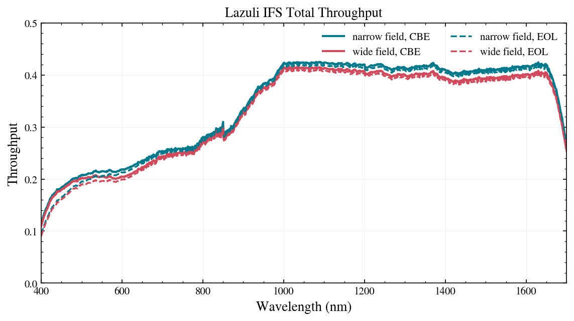
IFS total throughput for the narrow and wide fields in the CBE and EOL configurations
IFS total throughput in the narrow and wide fields, for the CBE and EOL estimates.

Transit spectroscopy beta

Transmission-spectrum simulator

The Transit spectroscopy page answers a different question from the ETC above: not the SNR of one exposure, but how well a transiting planet’s transmission spectrum can be measured with the IFS over one or more transits. It wraps lazuli_exo, which builds the atmosphere model and the host-star spectrum and asks slicersim for the per-wavelength noise.

GitHub ->
Reported quantities
σδ,λ= 2 SNRλ t14tramp Ntransits

The depth error per wavelength channel comes from the host star’s SNR in one readout ramp (the IFS ETC calculation, same field, frame time, jitter and background), scaled to the number of ramps that fit in the transit duration t14, with an equal out-of-transit baseline (the √2), and divided by √Ntransits. Channels are then binned to the requested resolving power R. The headline model-vs-flat S/N is the χ-distance between the noiseless model spectrum and a flat (Rp/R*)² line given those errors: a comparison metric for ranking targets and scenarios, not a calibrated detection significance.

Model assumptions

  • Atmosphere: isothermal H2/He equilibrium-chemistry model at Teq with metallicity [M/H] and C/O as free parameters, an optional gray cloud deck at a chosen pressure, and an optional power-law haze; the mean molecular weight follows the chemistry unless overridden. The scenario presets (clear, cloudy, high metallicity, hazy, flat) set these knobs. It is a comparison model, not a retrieval or a tailored prediction.
  • Host star: a PHOENIX model at Teff, log g and [Fe/H] (2000–8000 K; clamped outside the grid, blackbody below 2000 K), normalised to the magnitude, band and system you enter. Archive magnitudes are 2MASS J (Vega); slicersim works in AB and the conversion uses the band’s AB−Vega offset.
  • Readout: Auto starts from slicersim’s default MULTIACCUM ramp and halves the number of groups (then frames) until no detector pixel saturates on the host; a brighter host therefore gets a shorter ramp. Set N:M:D uses your readout as is and reports its saturation instead of removing it. The frame time, spectrograph field, jitter and zodiacal background are the ones you set; each ramp is repeated through the transit.
  • Noise: photon and read noise through slicersim only. No systematics floor, red noise, stellar activity, limb-darkening uncertainty or visit overheads. A result with saturated pixels is flagged and its errors are unreliable.
  • Light curves: illustrative white-light-style curves in three wavelength groups with quadratic limb darkening for hosts in lazuli_exo’s registry and a trapezoid otherwise.

Inputs and outputs

  • Planet lookup: typing a confirmed transiting planet fills the star (Teff, log g, [Fe/H], R*), the planet (Rp, Mp, Teq, transit duration) and the J magnitude from the NASA Exoplanet Archive composite table. Values the archive lacks are estimated and flagged in the banner: Teq from Teff and a/R* (zero albedo), the duration from a circular orbit, log g and [Fe/H] from solar defaults, and masses from the archive’s mass–radius relation.
  • Outputs: model-vs-flat S/N, median depth error per bin, feature amplitude, the readout used and ramps per transit; the binned spectrum with one noisy realization; light curves; a diagnostics table (scale height, μ, chemistry temperature, readout, saturated pixels); the host star’s one-ramp spectrum and SNR; and the up-the-ramp diagram.
  • Downloads: the binned curve as CSV (wavelength in µm, depth, 1σ error and the noisy realization per bin), the unbinned model curve, and the host star’s wavelength / flux / SNR traces. Depths are fractions.
  • Share links record every resolved input, including the readout mode and the instrument setup, so a link reproduces the run.

Site-wide notes

Scope and known limitations shared by all three calculators, the installed engine versions, and the link to the observatory documentation are on the site About page.